Consider this function:
$f(x) = x^4 - 4x + 10$
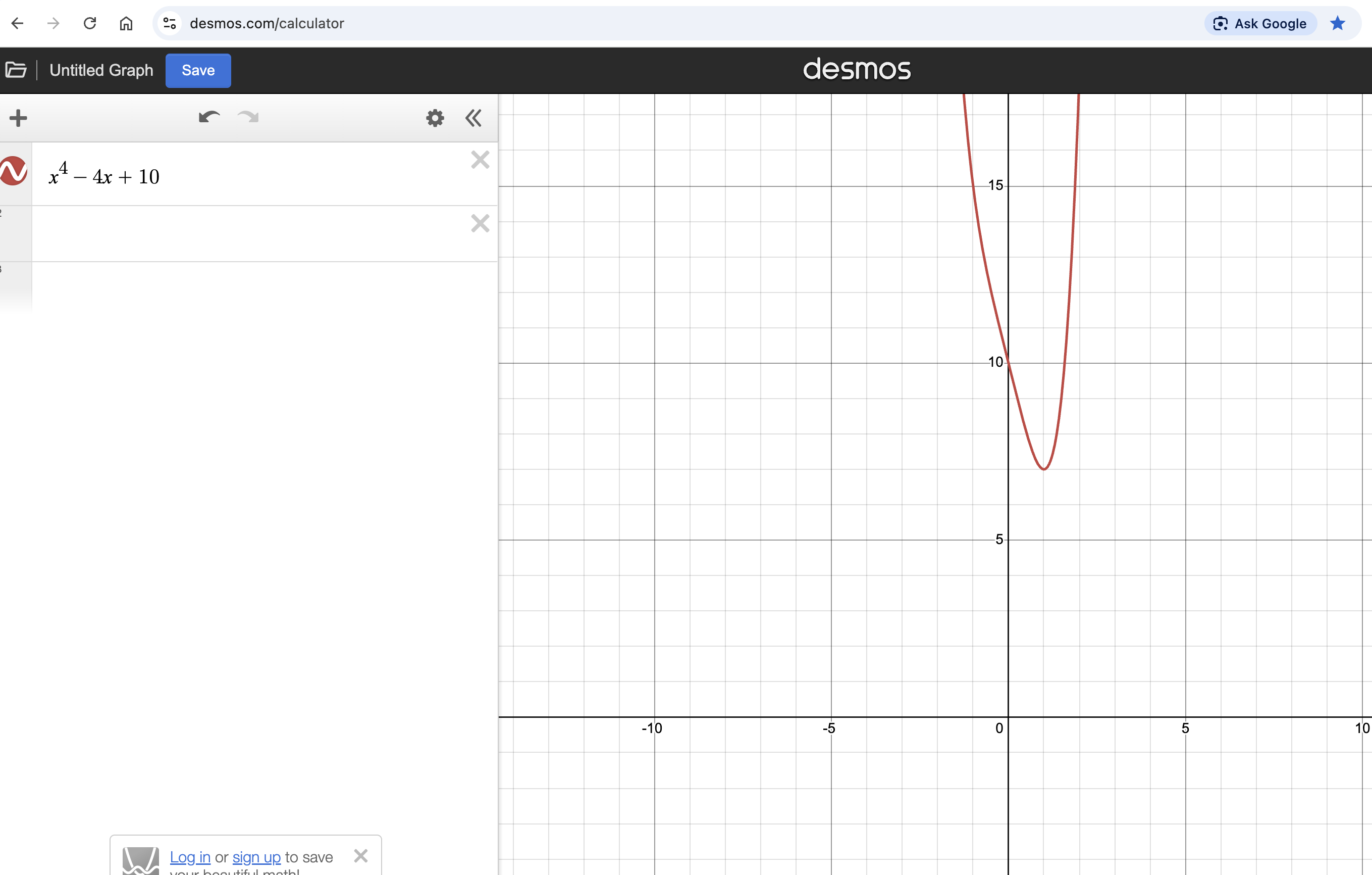
Go to desmos.com/calculator
and plot it. Type x^4 - 4x + 10 in the expression box.
Don’t just watch — invent.
What you’ll invent today:
And you’ll build it from scratch.
How this works:
Consider this function:
$f(x) = x^4 - 4x + 10$
Go to desmos.com/calculator
and plot it. Type x^4 - 4x + 10 in the expression box.
Notice the shape — it looks like a bowl.
A function is convex if it curves upward everywhere.
Visually: draw a straight line between any two points on the curve — the curve always stays below that line.
Is $f(x) = x^4 - 4x + 10$ convex?
Yes! It has a single valley — no bumps, no extra dips. A convex function has exactly one minimum.
Let’s work with this in Python. Write a function that computes $f(x) = x^4 - 4x + 10$:
def f(x):
    # your code here
def f(x):
return x**4 - 4*x + 10Call your function: what are f(-5) and f(5)?
| x | f(x) |
|---|---|
| −5 | 655 |
| 5 | 615 |
Both are large. The minimum is somewhere in between.
Can you find it?
Find the minimum by hit and trial.
Call f(x) for different values
in your notebook. Keep narrowing down.
How would you know you’ve reached the minimum?
Take a tiny step to the left and a tiny step to the right. If the function goes up on both sides — you’re at the bottom.
That’s exactly the right intuition: check whether the function is going up or going down near your point.
Now try another convex function:
$g(x) = x^2 - 2x + 5$
Find its minimum using hit and trial in Python.
The minimum is at x = 1, where g(1) = 4.
What strategy did you use? Describe it in words.
“Check a nearby value on each side. Move toward whichever side is lower. Keep going until neither side is lower.”
Convert your strategy into code:
def find_minimum(x):
    """
    Starting from x, find the value
    that minimizes f.
    """
    # your code here
Test it:
print(find_minimum(5.0))
# should print something close to 1.0
Your strategy works! But it’s slow — lots of tiny steps.
What if, instead of just checking left vs. right, you could know exactly how steep the function is and which direction is downhill?
That’s the slope.
At any point $x$ on the curve, the slope tells you:
| Slope positive (uphill to the right) | → move left |
| Slope negative (uphill to the left) | → move right |
| Slope zero | → you’re at the bottom! |
You know the slope of a line through two points: $\;\text{slope} = \frac{f(b) - f(a)}{b - a}$
To approximate the slope of the curve at $x$, use two points very close together:
$\text{slope at } x \;\approx\; \dfrac{f(x + h) - f(x - h)}{2h}$
where $h$ is a tiny number like $0.00001$.
Write this as a Python function:
def numerical_derivative(f, x, h=1e-5):
    """Return the slope of f at point x."""
    # your code here
def numerical_derivative(f, x, h=1e-5):
return (f(x + h) - f(x - h)) / (2 * h)Test on $f(x) = x^4 - 4x + 10$:
| x | Slope | Meaning |
|---|---|---|
| 0 | −4.0 | Negative → move right |
| 1 | ≈ 0 | Zero → at the bottom! |
| 2 | +28.0 | Positive → move left |
If the slope is positive, move left. If negative, move right. One formula captures both:
$x_{\text{new}} = x - \alpha \times \text{slope}$
$\alpha$ (alpha) is the step size — how far to move each time.
Hand-calculate one step. Start at $x = 2$, $\alpha = 0.01$:
| slope at $x = 2$ | = 28.0 |
| $x_{\text{new}} = 2 - 0.01 \times 28$ | = 1.72 |
| $f(1.72)$ | ≈ 11.9 (down from 18!) |
It moved downhill. One more step?
| slope at $x = 1.72$ | ≈ 16.4 |
| $x_{\text{new}} = 1.72 - 0.01 \times 16.4$ | ≈ 1.56 |
| $f(1.56)$ | ≈ 9.7 (still going down!) |
Keep stepping until the slope is near zero. Write this loop:
def find_minima_1d(f, x, alpha=0.01, epsilon=1e-6, max_steps=100000):
    """Return x that minimizes f, starting from the given x."""
    # Repeat: compute slope, update x
    # Stop when |slope| < epsilon
    # your code here
def find_minima_1d(f, x, alpha=0.01, epsilon=1e-6, max_steps=100000):
for step in range(max_steps):
slope = numerical_derivative(f, x)
if abs(slope) < epsilon:
break
x = x - alpha * slope
return x, f(x)find_minima_1d(f, x=2.0) → (1.0000, 7.0000)
Starting from $x = 2$, the algorithm walked to $x = 1$ — the exact minimum. This is gradient descent.
What happens if $\alpha$ is wrong?
$\alpha$ too large
Overshoots the minimum,
bounces back and forth,
may diverge
x: 2 → −6 → 200 → ∞
$\alpha$ just right
Steady progress
toward the minimum,
converges smoothly
x: 2 → 1.7 → 1.4 → 1.0
$\alpha$ too small
Barely moves,
takes forever,
may not converge in time
x: 2 → 1.997 → 1.994 → …
The learning rate $\alpha$ is the most important knob in gradient descent. Choosing it well is an art.
Now a function of two variables:
$g(x, y) = x^2 + y^2$
This is a bowl — a 2D landscape with a single valley at $(0, 0)$.
The slope now has two parts: how steep in the $x$ direction? How steep in $y$?
Same formula — hold one variable fixed, nudge the other:
$\dfrac{\partial g}{\partial x} \approx \dfrac{g(x\!+\!h,\; y) - g(x\!-\!h,\; y)}{2h}$ $\dfrac{\partial g}{\partial y} \approx \dfrac{g(x,\; y\!+\!h) - g(x,\; y\!-\!h)}{2h}$
These are called partial derivatives.
The update rule is the same — applied to each variable:
$x_{\text{new}} = x - \alpha \cdot \frac{\partial g}{\partial x}$ $y_{\text{new}} = y - \alpha \cdot \frac{\partial g}{\partial y}$
def find_minima_2d(g, x, y, alpha=0.01, epsilon=1e-6, max_steps=100000):
    """Find (x, y) that minimizes g."""
    # Repeat: compute partial derivatives, update x and y
    # Stop when gradient magnitude < epsilon
    # your code here
def find_minima_2d(g, x, y, alpha=0.01, epsilon=1e-6, max_steps=100000):
h = 1e-5
for step in range(max_steps):
dx = (g(x + h, y) - g(x - h, y)) / (2 * h)
dy = (g(x, y + h) - g(x, y - h)) / (2 * h)
if (dx**2 + dy**2)**0.5 < epsilon:
break
x = x - alpha * dx
y = y - alpha * dy
return x, y, g(x, y)find_minima_2d(g, 2.0, 3.0) → (0.0000, 0.0000, 0.0000) ✓
See the pattern?
| Position | Gradient | |
|---|---|---|
| 1D | a number | a number |
| 2D | a pair | a pair |
| ND | a list of N numbers | a list of N numbers |
One function handles all cases:
def compute_gradient(f, variables, h=1e-5):
    grad = []
    for i in range(len(variables)):
        v_plus = variables.copy();  v_plus[i] += h
        v_minus = variables.copy(); v_minus[i] -= h
        grad.append((f(v_plus) - f(v_minus)) / (2 * h))
    return grad

def find_minima(f, variables, alpha=0.01, epsilon=1e-6):
    variables = list(variables)
    for step in range(100000):
        grad = compute_gradient(f, variables)
        if sum(g**2 for g in grad)**0.5 < epsilon:
            break
        for i in range(len(variables)):
            variables[i] -= alpha * grad[i]
    return variables, f(variables)
One algorithm, any number of dimensions:
| Function | Start | Found minimum |
|---|---|---|
| $v_0^4 - 4v_0 + 10$ | [2.0] | ?[1.0] → f = 7.0 |
| $v_0^2 + v_1^2$ | [2.0, 3.0] | ?[0.0, 0.0] → f = 0.0 |
| $(v_0\!-\!1)^2 + (v_1\!-\!2)^2 + (v_2\!+\!3)^2$ | [0, 0, 0] | ?[1, 2, −3] → f = 0.0 |
You have built a general-purpose optimizer. It can find the minimum of any smooth function in any number of dimensions.
Now — what should we minimize?
You have data points. You want a line $y = mx + c$ that fits them.
Which line is best?
The red line
($m\!=\!1, c\!=\!5$) misses badly.
The green line
($m\!=\!2.5, c\!=\!4$) looks right.
But “looks right” isn’t a number.
How do you measure fit?
For each point, the line predicts $\hat{y}_i = m x_i + c$. The error is $y_i - \hat{y}_i$.
But some errors are positive and some negative — they cancel if you just add them.
How do you fix the cancellation problem?
Square each error (makes them all positive), then take the mean:
$\text{MSE}(m, c) = \frac{1}{N} \sum_{i=1}^{N} (y_i - (m x_i + c))^2$
A smaller MSE means a better fit. MSE = 0 means the line passes through every point.
Write the function:
def mse(X, y, m, c):
    """Mean Squared Error for the line y = mx + c."""
    # your code here
def mse(X, y, m, c):
total = 0.0
for i in range(len(X)):
predicted = m * X[i] + c
total += (y[i] - predicted) ** 2
return total / len(X)Test: $X = [1, 2, 3]$, $y = [3, 5, 7]$ — perfectly on the line $y = 2x + 1$:
| $(m, c)$ | MSE |
|---|---|
| (2, 1) | 0.0 — perfect fit |
| (1, 2) | 1.67 — close |
| (0, 0) | 27.67 — terrible |
MSE is a function of $m$ and $c$. What shape is its landscape?
A convex bowl — one single minimum.
You already have
find_minima.
MSE is just another function of two variables.
What if you plugged MSE into find_minima?
Wrap MSE so find_minima can use it
— it needs a function of a list:
def mse_for_optimizer(params):
    m, c = params
    return mse(X_data, y_data, m, c)

result, error = find_minima(mse_for_optimizer, [0.0, 0.0], alpha=0.001)
Found: m = 2.4970, c = 4.0189
True: m = 2.5, c = 4.0
This is linear regression.
You just built what
sklearn.linear_model.LinearRegression does.
Verify: np.polyfit(X_data, y_data, 1) uses an
exact formula (not gradient descent) and gives
the same answer.
So why use gradient descent at all?
The exact formula only works for linear models.
Gradient descent works for any differentiable function — including neural networks with millions of parameters.
The same loop you wrote — compute gradient, step, repeat — is how GPT, image classifiers, and AlphaFold are trained.
A house price depends on size and bedrooms and age. Give each feature its own slope:
$\hat{y} = m_0 x_0 + m_1 x_1 + \dots + m_{k-1} x_{k-1} + c$
def predict(x, m, c):
    """x: list of features, m: list of slopes, c: intercept."""
    # your code here
def predict(x, m, c):
total = c
for xi, mi in zip(x, m):
total += xi * mi
return totalpredict([1, 2], [2, 3], 1) → 9 # 2×1 + 3×2 + 1
The training loop is the same: compute gradient per weight, step against it.
def fit(X, y, learning_rate=0.01, epochs=5000):
    m = [0.0] * len(X[0])    # one weight per feature
    c = 0.0
    for epoch in range(epochs):
        grad_m, grad_c = gradients(X, y, m, c)
        for i in range(len(m)):
            m[i] -= learning_rate * grad_m[i]
        c -= learning_rate * grad_c
    return m, c
Test on $y = 2x_0 + 3x_1 + 1$:
X = [[1,2], [2,1], [3,4], [4,3]]
y = [9, 8, 19, 18]
fit(X, y) → m = [2.000, 3.000], c = 1.000 ✓
Same algorithm. More weights. That’s it.
What if the data follows $y = x^2$? A straight line can’t fit a curve.
X = [[1],[2],[3],[4],[5]],
y = [1, 4, 9, 16, 25]
fit(X, y) → MSE > 1 (stuck!)
The escape: add a column. If $y = x^2$, then as a function of $x^2$ it’s a straight line!
def add_feature(X, fn):
    return [row + [fn(row)] for row in X]

X2 = add_feature(X, lambda row: row[0]**2)
# X2 = [[1,1], [2,4], [3,9], [4,16], [5,25]]
fit(X2, y) → MSE < 0.01 ✓
Same algorithm, no new math. You added the right feature, and the linear model handled the rest.
Before deep learning, this was most of the job of a machine-learning engineer.
What you built:
| 1. | numerical_derivative | — slope at a point |
| 2. | find_minima | — walk downhill to the bottom |
| 3. | mse | — measure how wrong a line is |
| 4. | find_minima(mse) | — linear regression! |
| 5. | predict + fit | — many features, same algorithm |
| 6. | add_feature | — fit non-linear data |
What’s next?
Replace $\hat{y} = mx + c$ with a neural network — the gradient descent loop stays exactly the same, but the model becomes vastly more powerful. That’s deep learning.